3 Theory & tools & observation of Turbulence

1 Turbulence: The legacy of A.N. Kolmogorov

Frisch, U. (1995). Turbulence: The legacy of A.N. Kolmogorov. Cambridge University Press. https://doi.org/10.1017/CBO9780511623343

2 A Practical Guide to Wavelet Analysis (read partially)

Torrence, C., & Compo, G. P. (1998). A practical guide to wavelet analysis. Bulletin of the American Meteorological Society, 79(1), 61-78. doi: 10.1175/1520-0477(1998)079<0061:APGTWA>2.0.CO;2

2.1 简介

通过大气科学中的 El Niño–Southern Oscillation (ENSO) 现象的例子，给出了一个实用的小波变换(Wavelet Analysis)过程的指南，并包含统计显著性检验。

2.1.1 Wavelet analysis

WFT(Windowed Fourier transform) 是一种从信号中提取局部频率信息的分析工具，Window 指的是 sliding segment

对 $f (t)$ 做小波变换:

W (τ, t) = \sum_{i = 0}^{N - 1} f (t_{i}) ψ^{*} [(t_{i} - t) / τ] = \frac{1}{\sqrt{| τ |}} \int_{- \infty}^{\infty} f (x) ψ^{*} (t - x) d x, ψ (u) = 2^{1 / 2} π^{- 1 / 4} \cos (ω_{0} u) \exp (- u^{2} / 2),

可见尺度 $τ$ 影响母函数, 进而调制 $ψ$ , 动态调整窗口大小, $τ$ 小 $ψ$ 被压缩为高频小波: 高频窄窗高时间分辨率，低频宽窗高频率分辨率. 而 $W F T$ 固定窗口大小 $T$ ，时频分辨率固定不可调:

F (ω, t) = \int_{- \infty}^{\infty} \underset{W i n d o w F u n c t i o n}{\underset{⏟}{w (x - t)}} f (x) e^{- i ω x} d x

note:

在时间序列两端进行零填充，可以一定程度上减小影响锥(Cone of influence (COI))范围(section 3g);
一般选取指数尺度集 $s_{j} = s_{m i n} 2^{j δ j}$ ，对于莫雷小波 $δ j \leq 0.5$ ， $s_{0}$ 应选择使等效傅立叶周期近似为 $2 δ t$ (section 3f & 3h);
重构(section 3i)

\begin{matrix} (1) & x_{n} = \frac{δ j δ t^{1 / 2}}{C_{δ} ψ_{0} (0)} \sum_{j = 0}^{J} \frac{ℜ {W_{n} (s_{j})}}{s_{j}^{1 / 2}} \end{matrix}

$x_{n}$ 的方差是(类似于 Fourier 变换的 Parseval 等式)：

\begin{matrix} (2) & σ^{2} = \frac{δ j δ t}{C_{δ} N} \sum_{n = 0}^{N - 1} \sum_{j = 0}^{J} \frac{{| W_{n} (s_{j}) |}^{2}}{s_{j}} \end{matrix}

2.1.2 理论功率谱和显著性检验水平

红噪声和白噪声

To determine significance levels for either Fourier or wavelet spectra, one first needs to choose an appropriate background spectrum. It is then assumed that different realizations of the geophysical process will be randomly distributed about this mean or expected background, and the actual spectrum can be compared against this random distribution. For many geophysical phenomena, an appropriate background spectrum is either white noise (with a flat Fourier spectrum) or red noise (increasing power with decreasing frequency).

一个红噪声的简单模型是单变量滞后自回归(univariate lag-1 autoregressive)：

\begin{matrix} (3) & x_{n} = α x_{n - 1} + z_{n}, x_{0} = 0, z_{n} \in {Guassian white noise} \end{matrix}

$α$ 決定序列中相邻数据点之间的关联程度(“红”度)。除以 $\frac{N}{2 σ^{2}}$ 归一化得到噪声谱：

\begin{matrix} (4) & P_{k} = \frac{1 - α^{2}}{1 + α^{2} - 2 α \cos (2 π k / N)} \end{matrix}

lag-2 红噪同理。若上述噪声回归方程是全局的，则是傅里叶红噪声。可以使局域/很小的垂直切片满足(3)式，得到小波红噪声谱。

零假设和显著性水平

The null hypothesis is defined for the wavelet power spectrum as follows: It is assumed that the time series has a mean power spectrum, possibly given by (4); if a peak in the wavelet power spectrum is significantly above this background spectrum, then it can be assumed to be a true feature with a certain percent confidence. For definitions, “significant at the 5% level” is equivalent to “the 95% confidence level,” and implies a test against a certain background level, while the “95% confidence interval” refers to the range of confidence about a given value.

2.2 链接

本地 2.2 A Practical Guide to Wavelet Analysis

2.3 补充

词汇 _Documents/words/Part.3 words#2 A practical guide to wavelet analysis

3 Characterization of turbulence in the Mars plasma environment with MAVEN observations (partially)

Ruhunusiri, S., et al. (2017), Characterization of turbulence in the Mars plasma environment with MAVEN observations, J. Geophys. Res. Space Physics, 122, 656–674, doi:10.1002/2016JA023456.

3.1 简介

摘要

我们首次通过计算磁场波动(magnetic field fluctuations)的谱指数(slopes in the magnetic field power spectra)并确定它们随频率和在不同区域的变化，来表征火星等离子体环境中的湍流。

与太阳风不同，在磁鞘中，我们发现惯性区缺失(an absence of the inertial range)，该区域的谱指数值等于科尔莫戈罗夫定标值 $- 5 / 3$ 。相反，正如在其他行星的磁鞘中观察到的那样，我们发现谱指数从低频(低于质子回旋频率(gyrofrequency))的接近 $- 0.5$ 的低负值过渡到高频(高于质子回旋频率)的远低于 $- 5 / 3$ 的值。这表明原始太阳风(pristine solar wind)在火星弓激波处被改变，并且波动主要由磁鞘中局部产生的波动主导。

缺乏具有科尔莫戈罗夫定标值的谱指数表明，磁鞘中的波动没有足够的时间相互作用，从而未能导致充分发展的能量级联(a fully developed energy cascade)。

在磁场堆积边界(magnetic pileup boundary, MPB)附近，低频范围观察到接近科尔莫戈罗夫定标值的谱指数，这表明存在充分发展的能量级联。

在尾迹(wake，不是磁尾 magnetic tail)中，我们发现低频和高频范围的谱指数大致相同，通常接近 $- 2$ 。

我们观察到谱指数的季节性变化，主要在上游区域，这表明质子回旋波(proton cyclotron waves)存在季节性变化。

3.1.1 背景介绍

3.1.2 方法

refer to the lower frequency range ( $< f_{H^{+}}$ ) as the MHD range and the higher frequency range ( $> f_{H^{+}}$ ) as the kinetic range.
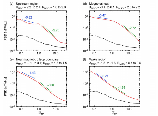
使用小波变换得到幂律谱(power spectral densities (PSDs) for the magnetic field fluctuations)

PSD (f) = \frac{2 Δ t}{N} \sum_{j = 1}^{N} {| W_{x} (t_{j}, f) |}^{2} + {| W_{y} (t_{j}, f) |}^{2} + {| W_{z} (t_{j}, f) |}^{2}

借助积累的数据和网格划分，得到数据密度和本地质子回旋频率 $f_{H^{+}}$ (中位数)的分布：

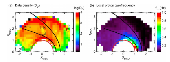
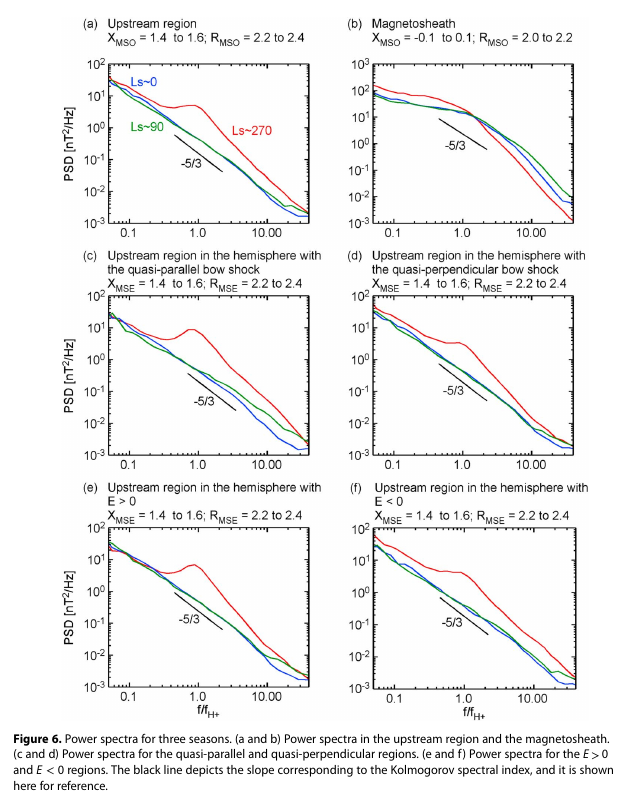
绘制上图选取的几个具有代表性的网格单元的谱 PSD (下图的 cdef 对应上图的 bcde 单元, 这是文章的绘图编号错误)

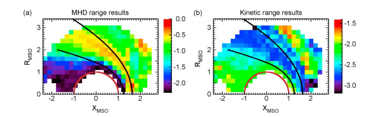
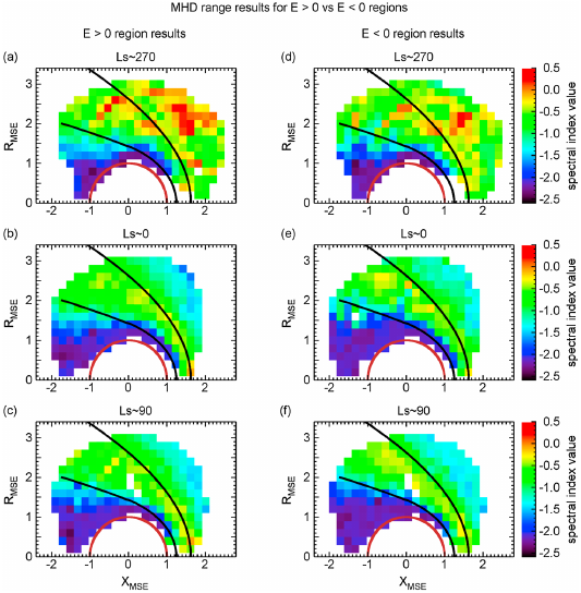
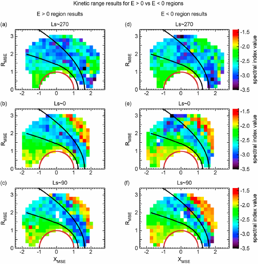
以及 spectral index value 的空间分布

谱斜率的时间分布

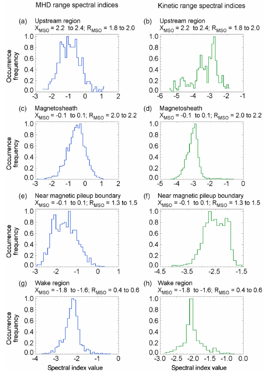
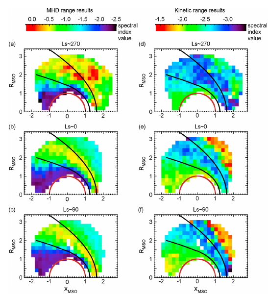
根据太阳黄经 Ls (Solar Longitude)： $L s = 0^{\circ}, 90^{\circ}, 180^{\circ}, 270^{\circ}$ ：春分/夏至/秋分/冬至（北半球春/夏/秋/冬季开始），可以绘制谱的季节变化：

可见

The MHD range spectral indices show seasonal variability in the upstream region and in the magneto-sheath, while the kinetic range spectral indices show seasonal variability in the upstream region and in the night-side magnetic pileup region.

这是因为

During these times( $L s = 0^{\circ}, 90^{\circ}, 180^{\circ}, 270^{\circ}$ ) the distance from Sun to Mars is approximately 1.56, 1.65, 1.45, and 1.38 AU, respectively. Due to the changes in the distance between Mars and the Sun, the solar EUV flux at Mars varies seasonally (差值约达 $\propto {(\frac{r_{Aphelion}}{r_{Perihelion}})}^{2} - 1 = {(\frac{2.492 \times 10^{8} km}{2.067 \times 10^{8} km})}^{2} \approx (1.205)^{2} - 1 \approx 45 %$ ), and the exospheric density varies accordingly.

特定区域的谱的季节变化:

这表明前面那个编号错误的图的第一行两个子图，只是上图的第一行的两个子图中 $L s = 270^{\circ}$ 的特例，即距离太阳最近的时刻。 $E$ 为 the upstream electric field refers to the upstream convection electric field given by $E = - V_{S W} \times B_{I M F, u p s t r e a m}$ ，文章关注 asymmetry，所以 $E > 0$ 实际上是 $Z_{M S E} > 0$ 。

newly born pickup ions should preferentially excite upstream waves in the positive electric field side.

refer to [section 5]:

Closer to Mars, protons are created by photoionization, charge exchange, and electron impact ionization of the neutral hydrogen exosphere. These ions are subsequently accelerated in the upstream solar wind electric field direction and neutralized by charge exchange due to the collisions with the neutral exospheric atoms. These drifting neutrals, which are prominently in the E > 0 region, then undergo ionizations forming newly born pickup ions which excite proton cyclotron waves preferentially in the E > 0 region [Russell et al., 2006]. Thus, if the waves are generated by mechanism 2 mentioned above, they should occur more frequently in the E > 0 hemisphere.

谱噪声估计

we verified that the PSDs used for computing the median lie above the MAG noise level, shown by the black curves in Figures 3c–3f(即上面编号错误的图中的黑色曲线). The MAG noise level was estimated as the minimum PSD value when MAVEN was upstream of the bow shock during the time interval from November 2014 to April 2016.

the sign of $B_{X M S E}$ or the X − MSE component of the magnetic field is indicative of the foreshock locations.

$θ = ⟨ B, X_{M S E} ⟩$ , When $B_{X M S E} > 0$ or when $0^{\circ} < θ < 90^{\circ}$ the quasi-parallel shock(where $⟨ \vec{n}, \vec{B} ⟩ \in [0^{\circ}, 45^{\circ}]$ ) or the foreshock region is located at $Y_{M S E} > 0$ , whereas the quasi-perpendicular shock region is located at $Y_{M S E} < 0$ . When $B_{X M S E} < 0$ or when $90^{\circ} < θ < 180^{\circ}$ the quasi-parallel shock region is located at $Y_{M S E} < 0$ , whereas the quasi-perpendicular shock region is located at $Y_{M S E} > 0$ .

In the quasi-parallel region we expect enhanced perturbations due to the generation of waves via bow shock reflected solar wind ions (the waves are generated efficiently when the particle populations back stream quasi-parallel to the magnetic field [Gary, 1991]) and also reflected pickup ions from Mars’ extended hydrogen exosphere.

在考虑不同区域的网格划分、MHD/Kinetic 尺度、季节变化之后，继续添加：准垂直/平行约束或者 $E < 0 o r E > 0$ 的区分，就得到



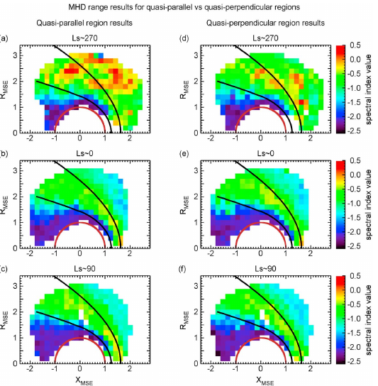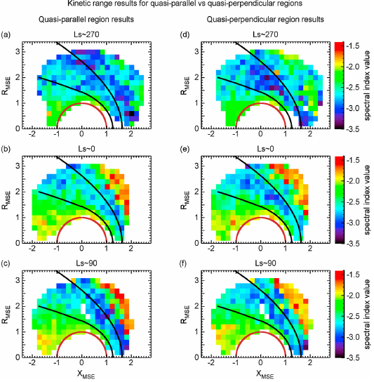发现两者很相似。

3.1.3 讨论

在太阳风的 MHD range 中，谱斜率的典型值为 $- \frac{5}{3}$ 。对于 $L s = 0^{\circ}, 90^{\circ}$ 的 upstream region 的确接近该值，但谱斜率仍然 takes a wide range，因为

The quasi-parallel region can be highly disturbed due to the presence of proton cyclotron waves that can be excited by reflected solar wind protons from the bow shock. Since Mars also has an extended hydrogen exosphere which can give rise to pickup proton populations upstream of Mars, it can also contribute to the generation of upstream proton cyclotron waves. The median magnetic field spectra computed in the upstream region contain all these contributing effects

在太阳风的 Kinetic range 中，谱斜率的典型值为 $- 2.8$ [Sahraoui et al., 2010; Roberts et al., 2013; Sahraoui et al., 2013; Roberts et al., 2015]。观测与之相近却不完全一致，These differences should be a consequence of Mars upstream phenomena which perturb the turbulence characteristics of the pristine solar wind.

3.2 补充

词汇 Part.3 words

3.3 链接

本地 3.3 Ruhunusiri et al_2017_Characterization of turbulence in the Mars plasma environment with MAVEN

4 The solar wind interaction with Mars Locations and shapes of the bow shock

Vigne. D., et al. (2017), The solar wind interaction with Mars Locations and shapes of the bow shock, GEOPHYSICAL RESEARCH LETTERS, 27(1), 49-52.

5 Quantitative Prediction of High-Energy Electron Integral Flux at Geostationary Orbit Based on Deep Learning

Wei, L., Zhong, Q., Lin, R., Wang, J., Liu, S., & Cao, Y. (2018). Quantitative prediction of high-energy electron integral flux at geostationary orbit based on deep learning. Space Weather, 16, 903–916. https://doi.org/10.1029/2018SW001829

5.1 简介

5.1.1 recurrent neural network (RNN)

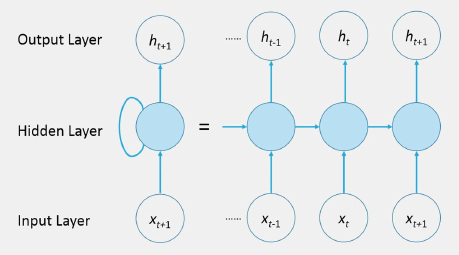
Unlike traditional feed-forward neural networks, RNNs add loops in themselves, allowing information to be retained from a previous time to the next by iterative function loops
The back-propagation trough time algorithm is used to adjust and renew the network parameters during the training process (residual calculation).
equation:

h_{t} = σ (W_{x h} x_{t} + W_{h h} h_{t - 1} + b)

a gradient vanishing and explosion problem exists if the input sequence is too long

5.1.2 Long Short-Term Memory (LSTM)

LSTM repeating module architecture	Meaning	Formulas
!401	$x_{t}$ : Input at moment $t$ $h_{t}$ : Output $C_{t}$ : Cell state ${\tilde{C}}_{t}$ : Candidate values $f_{t}$ : Forget gate function $i_{t}$ : Input gate function $o_{t}$ : Output gate function $σ, \tanh$ : Activation function Blue circles: Neural network layers $\times$ : Element-wise Multiplication ' $*$ '	$$\begin{array}c\begin{array}c f_t = \sigma(W_f \cdot [h_{t-1},x_t] + b_f)\ i_t = \sigma(W_i\cdot [h_{t-1},x_t] + b_i) \ \widetilde{C}t = \tanh(W_c\cdot [h,x_t] + b_C) \ C_t = f_t * C_{t-1} + i_t * \widetilde{C}_t \ o_t = \sigma(W_o \cdot [h_t-1,x_t] + b_o) \ h_t = o_t * \tanh(C_t) \end{array} \[8pt] \begin{cases} \sigma(x) = \frac{1}{1+e^{-x}} \[3pt] \tanh(x) = \frac{{1-e^{-2x}}}{1+e^{-2x}} \end{cases}\end{array}$$

LSTM layer principle ex.

Data Structure and Batch Processing
For time series [1,2,3,4,5], splitting to X=[[1,2],[2,3],[3,4],[4,5]] and y=[3,4,5,6]:

X contains 4 samples (batch_size=4), each sample is a sequence of length 2(time_step=2), and input_size=1 for 1D data series
The model processes these samples in batches, performing forward propagation independently for each sample
Taking the first sample [1, 2] as an example, the LSTM processing steps:
1. Time step 1: Process input 1, update hidden state h1
2. Time step 2: Process input 2, combine with h1 to update hidden state h2
3. Extract features: Take the hidden state from the last time step h2
4. Prediction: Map h2 to a predicted value through a linear layer, compare with target value 3

Parallelism in Batch Processing

The model processes multiple samples simultaneously (depending on batch_size)
For all 4 samples in X, the LSTM executes the above processing steps in parallel
The processing of each sample is independent, and ultimately each sample yields a predicted value

5.1.3 Calibration

The logarithm of the daily electron integral flux from the three pairs of GOES satellites during the overlapped period has strong. linear correlations. Based on this, the values from different satellites are calibrated using the data of GOES-11 by using the method of linear fitting that covers the time period from January 1999 to December 2016.

In addition, piecewise linear fitting is used to calibrate the data from GOES-13 to GOES-11.

5.1.4 Model Result

Spearman’s rank correlation analysis

Unlike the more common Pearson correlation, which looks for linear relationships (straight lines), Spearman looks for monotonic relationships. This means it checks if, as one variable increases, the other tends to increase (corr>0) or decrease(corr<0), even if that change isn't a perfectly straight line.

For a dataset without many tied ranks, the formula is:

r_{s} = 1 - \frac{6 \sum d_{i}^{2}}{n (n^{2} - 1)} = 1 - \frac{2 \sum d_{i}^{2}}{\sum i^{2}} \in [- 1, 1]

$d_{i}$ is the difference between the ranks of each observation.
$n$ is the number of observations.

How to Calculate it in Python:

# Offset Time: Shifting 'sales' back by 2 periods
df['sales_lagged'] = df['sales'].shift(-2)

# Using scipy
from scipy import stats
x = [10, 20, 30, 40, 50]
y = [2, 2.4, 10, 8, 25]
coef, p_value = stats.spearmanr(x, y)
print(f"Spearman Correlation Coefficient: {coef:.3f}")
print(f"P-value: {p_value:.3f}")

# Using pandas for DataFrame
import pandas as pd
df = pd.DataFrame({'study_hours': [1, 5, 2, 8, 4], 'test_scores': [50, 88, 60, 95, 78]})
correlation_matrix = df.corr(method='spearman')
print(correlation_matrix)

result:
!696
According to the correlation, the ﬂux itself, solar wind velocity, Dst, and Kp indices are considered to be better input factors for modeling. The remaining parameters, with the exception of IMF, are also used as inputs for modeling.

The feature of offset time is an important factor of setting the time step in modeling to determine the number of consecutive days to be used as inputs to the model.

5.1.5 Daily-Based Model

5.1.6 Hourly-Based Model

5.2 补充

Part.3 words

5.3 链接

本地 3.5 Wei et al. - 2018 - Quantitative Prediction of High-Energy Electron Integral Flux at Geostationary Orbit Based on Deep Learning